How large is this? see next subtopics

Try this out at the playground, or the Del Mar Fair, or on a lazy susan.

2. Large-scale flow with Coriolis force

Coriolis Force Acceleration = 2 omega (sin 45)v = 2 x (2 pi/86400)x 0.707 x 100 = 10^-2 to the east.

They balance! This will be important.

2.b. Coriolis force alone. Start motion impulsively - thereafter if Coriolis is the only force, acceleration is always to the right of the motion. So the motion veers.

Equations for Coriolis force become necessary at this point:

(figure) and period T = (2 pi)/(2 omega sin latitude) = (12 hr)/sin latitude
We see motion like this very frequently in moored current meter records - at the local "inertial period" which is 12 hr/sin latitude with a little spread about this period. What is the inertial period at different latitudes? (pole, 45 degrees, 30 degrees, equator).

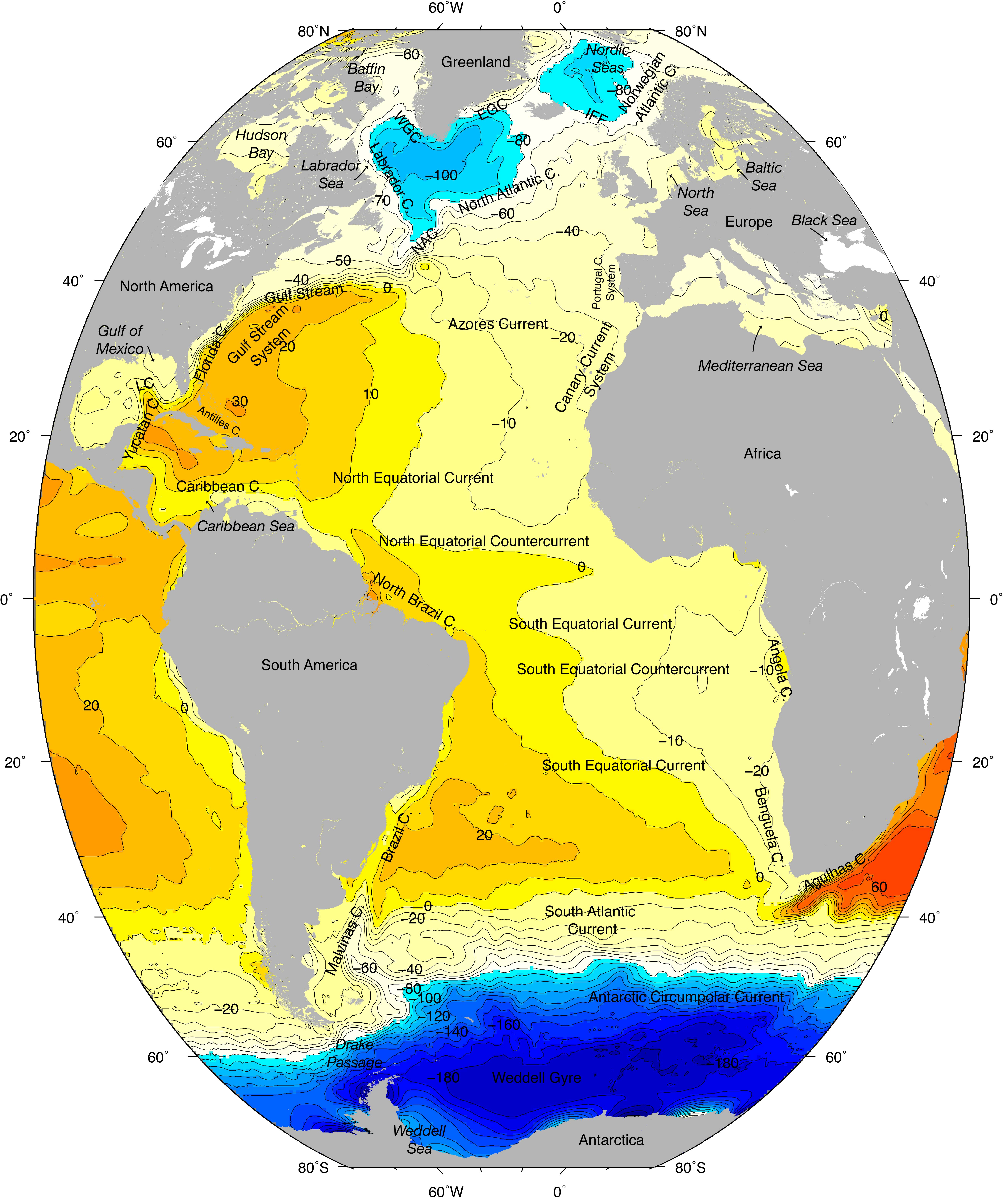
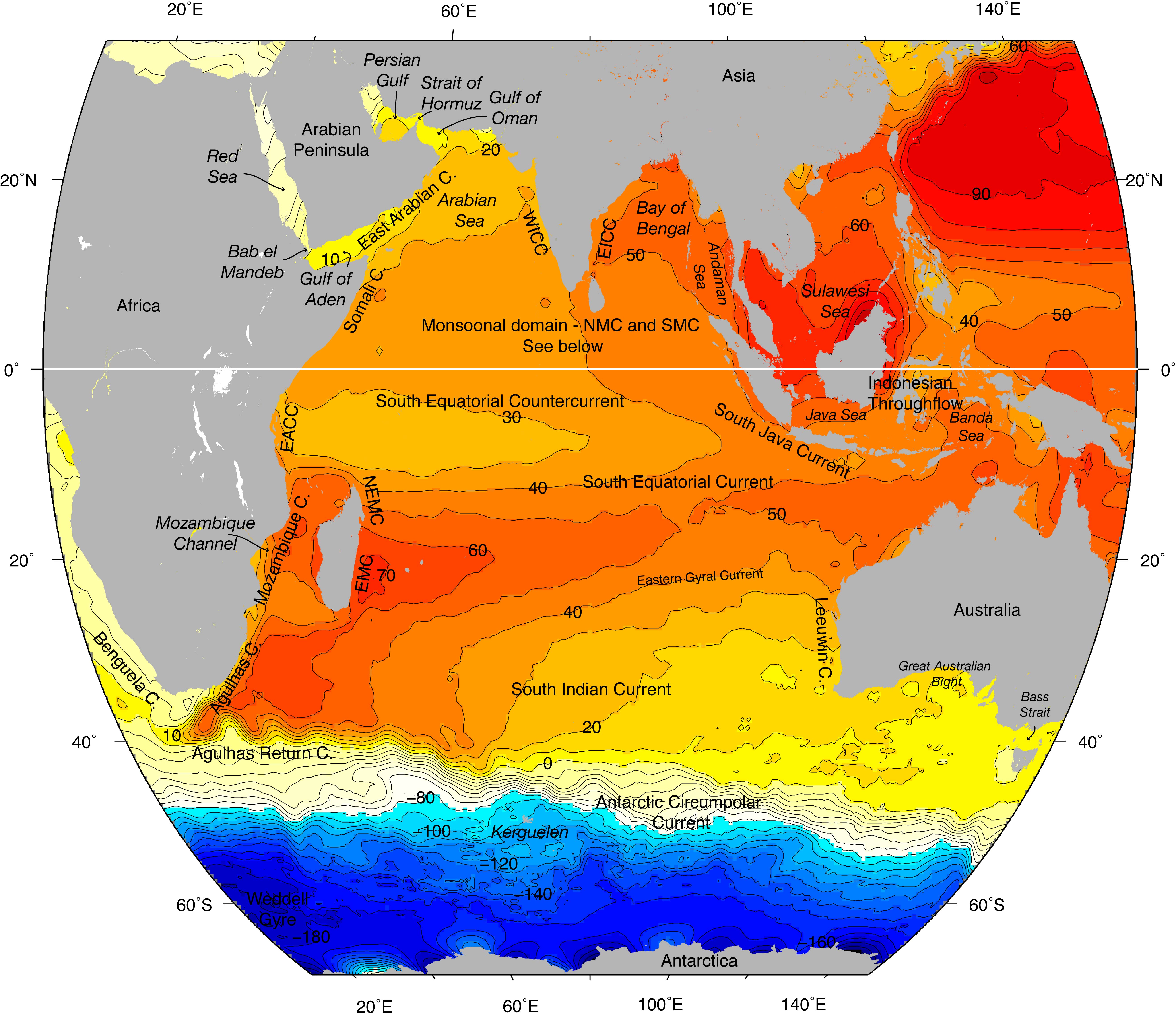
2.c. Geostrophic/ weathermap flow

On a weathermap around a high pressure center:

Meteorologists measure pressure at different locations, and then use the balance PGF = (2 omega sin latitude)speed to get the wind speed. This balance is called geostrophic flow. That is, they can interpret the pressure maps for the winds. This is why oceanographers also want to measure pressure, since the same holds in the ocean.

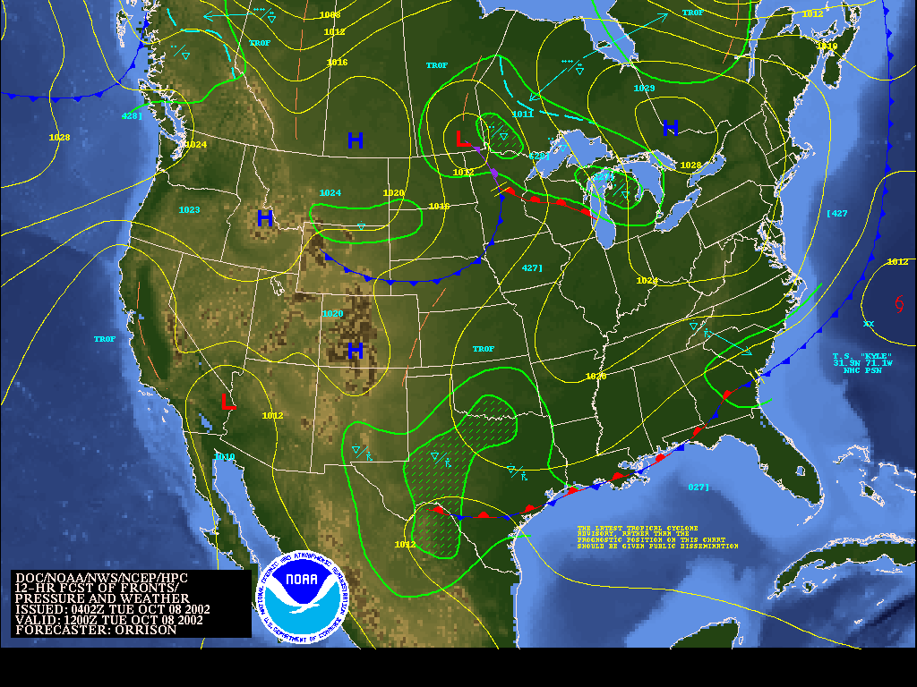
Weather map for the U.S. for October 8, 2002 from the National Weather Service.

But as we've seen before, oceanographers cannot usually measure pressure differences well enough to obtain the PGF that goes with geostrophic flow (see section 3 below). Even with satellite altimeters that measure the sea surface height pretty well, the error is still several centimeters (with the limitation being the accuracy of the geoid). So oceanographers measure fluid density rho(x,y,z). They then use the hydrostatic balance to figure out the pressure at each depth, based on the mass of fluid above that depth. That is:

PGF_{one_depth} - PGF_{another_depth} = (2 omega sin latitude)(speed_{one_depth} - speed_{another_depth})

Oceanographers either draw such maps, say the flow at the surface relative to 1000 dbar for instance, or look at sections to see the difference in speeds.

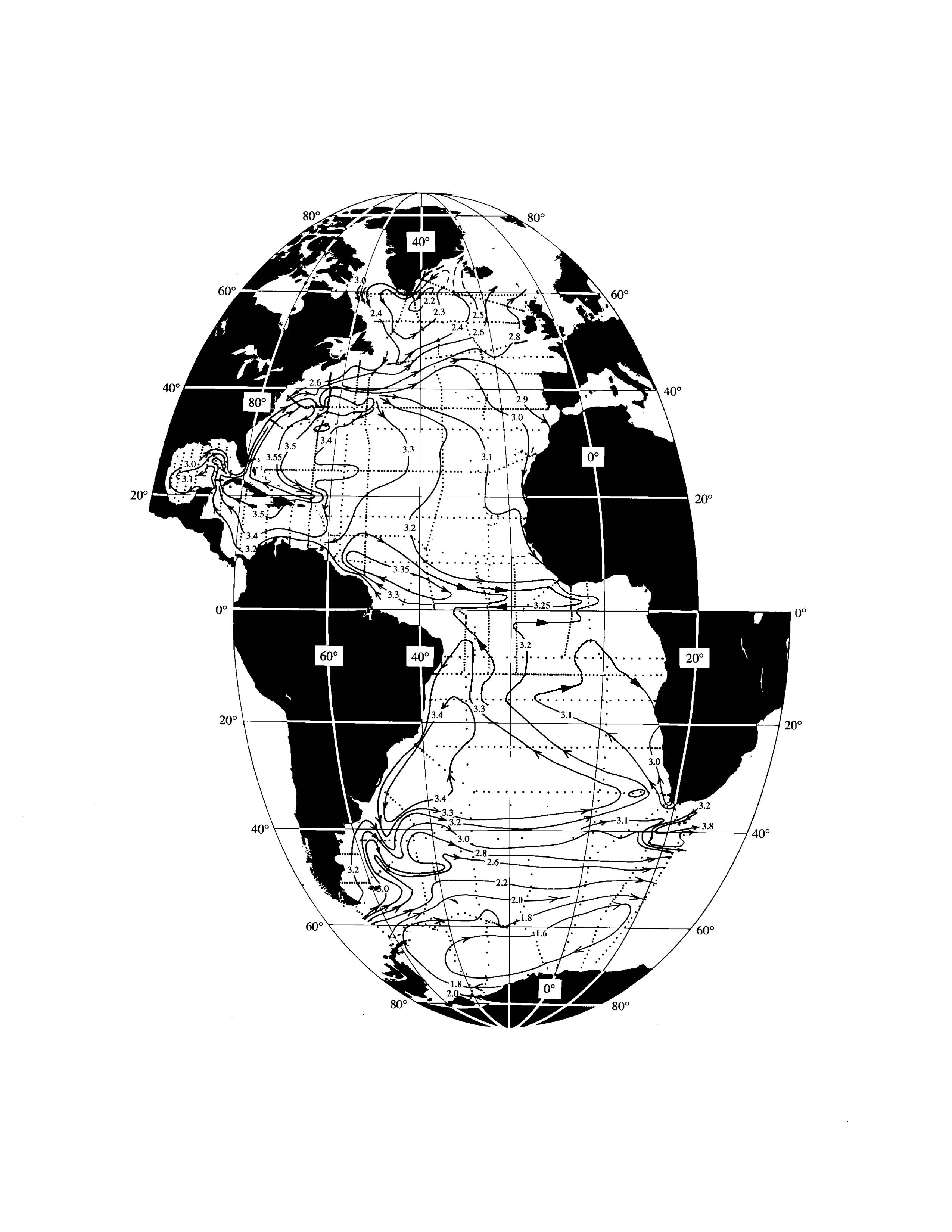
Atlantic surface height (steric height, something like dynamic height) from Reid (1994).
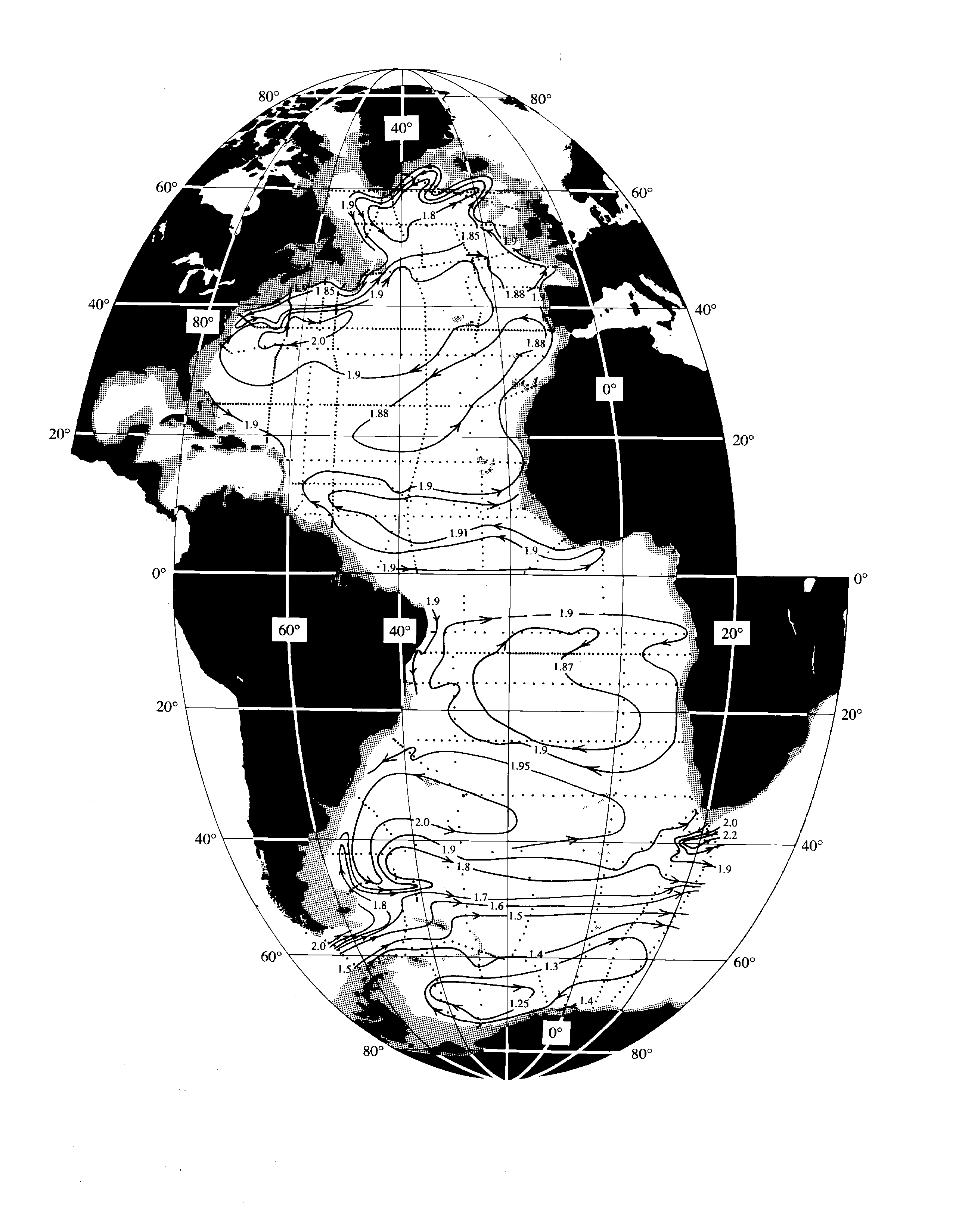
Atlantic 1000 dbar (steric height, something like dynamic height) from Reid (1994).

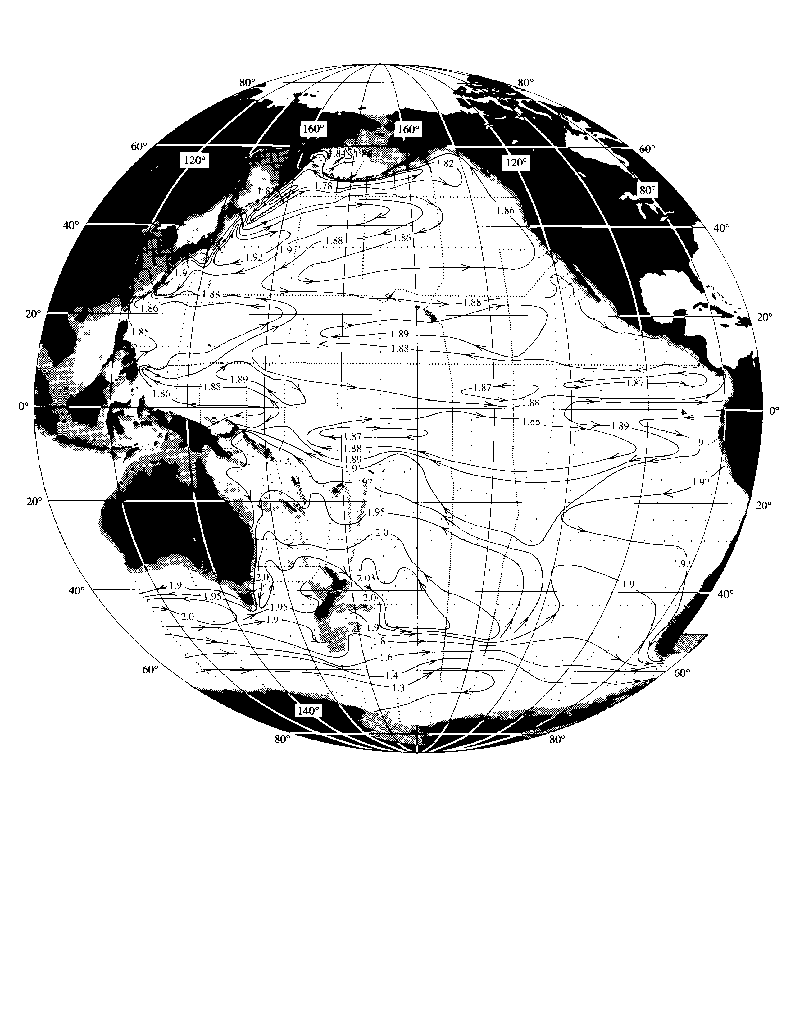
Pacific surface height (steric height, something like dynamic height) from Reid (1998).
Pacific 1000 dbar (steric height, something like dynamic height) from Reid (1998).
Note the high and low pressure regions. Note how much smaller the basin-scale pressure gradient force is at 1000 dbar compared with 0 dbar.

(Talley extra: If oceanographers have more information - say, they have measured the flow at one depth using something like a subsurface float deployment, or if they infer the flow at one depth using something like tracer patterns, and perhaps combine these patterns with strong constraints on how much total transport can move through some particular region, they can work out the absolute flow field. This is quite a difficult endeavor. We will look at some examples of such solutions.)

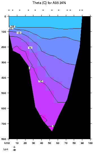
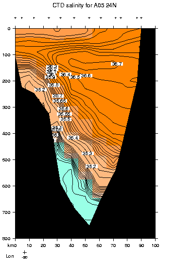
Example of a section across the Gulf Stream:

1. Measure temperature and salinity and compute the density. Across the Gulf Stream, we see isopycnals plunging hundreds of meters from on to offshore (towards the east if looking at an east-west section).
2. As one guess, assume there is no flow at some depth, which means that the PGF = 0 at that depth. This was common practice until about 20 years ago, and the depth assumed with no flow was called the "level of no motion". (In reality, there is almost never such a level, but this is a convenient step for teaching how to compute relative speeds.)
3. Go upward from that level where PGF = 0 on the west side, which is the cold, dense side and calculate how the pressure decreases as you go up. Then go upward from the PGF=0 level on the east side, which is warm and less dense and calculate the pressure decrease. The pressure will decrease faster on the cold, dense side since the water is heavier and more is subtracted at each step.
4. Therefore at a higher level, the nearshore (cold, dense) P < offshore (warm, light) P. Therefore the PGF is westward at all of these higher levels, above the PGF = 0.
5. If the flow is geostrophic, which we assert, the Coriolis force is eastward. Therefore the flow is northward.
6. Since the Pressure gradient persists to the very surface, the surface itself must slope upward from west to east so that the pressure is higher offshore. If in fact we could measure the sea surface height relative to the geoid, this is what we would find (and which is found in various interpretations of satellite altimetry data).
7. Caveat: we don't really know what the PGF is at a given depth; we just assumed PGF = 0 at some depth since we expect from other observations that the flow is much weaker at depth than at the surface in the Gulf Stream. All that we actually know from measuring the density is the relative flow at one depth compared with another - that is, we know the geostrophic velocity shear and not the absolute geostrophic flow.

Figure: Gulf Stream potential density section
Figure: Gulf Stream potential temperature section
Figure: Gulf Stream salinity section
at 26N, Florida Strait, in August, 1981

3. Dynamical quantities for the general circulation. (modified from Talley, 2000 lecture notes)

Direct current measurements - require time and space averaging and/or filtering to remove unwanted signals such as those from tides and internal waves. The remaining signal still contains all of the time scales of the large-scale circulation. It is more or less the case that long time scales go with large horizontal spatial scales. There is no hard and fast rule about how long the time average must be that corresponds with a velocity estimate associated with the pressure gradient. (current meter results, float trajectories and averages.)

Pressure gradients are used to calculate geostrophic flows, as described above. Pressure can be measured in several ways. Altimetry provides the sea surface height to within several centimeters, which is not adequate for the "mean" circulation, but is adequate for determining the variability of the surface currents about an unknown mean. Pressure gauges on the ocean bottom can be calibrated with direct current measurements (say from current meters), and then used in pairs to calculate geostrophic flow. As with direct current measurements, time series signals must be averaged or filtered.

Finally, pressure gradients can be determined from dynamic height (density field), again to within an unknown pressure at each position (as described above, and below). The unknown can be thought of as due to the unknown exact sea surface height relative to the geoid (and which altimetry is mainly not quite adequate to measure).

Velocities associated with the general circulation are then mostly calculated from the pressure gradients.

3.2 Dynamic height. To calculate pressure at a point relative to a deeper or shallower point at the same horizontal location, from the measured density field, using the concepts outlined above.

Use hydrostatic balance, which is the force balance between the vertical pressure gradient and gravity*density.

Dynamic height is an historical quantity, which means that its definition includes some anachronisms owing to the way it had to be calcaulted prior to computers. Define dynamic height D such that

10 delta D = g delta z
10(D₂ - D₁) = g (integral from 1 to 2) dz

If delta z = 1 meter, delta D = (g delta z)/10 <~ 1 m²/sec² = 1 dynamic meter (definition).

To calculate D from density, use the hydrostatice relation: 0 = -alpha dp - g dz. Then D = -(1/10)integral (from p₁ to p₂) alpha dp', in units of dynamic meters. You see here how the density comes in to work out the pressure change from one depth to another.

For practical purposes, people often use "delta D" instead of "D": alpha = alpha_35,0,p + del where del = specific volume anomaly. Then delta D = = -(1/10)integral (from p₁ to p₂) del dp'

The geostrophic velocity is then obtained in terms of dynamic height:
fv = 10 (d/dx)(delta D) and fu = -10 (d/dy)(delta D)
where f is the Coriolis parameter defined before: 2 omega sin(latitude), x and y are the east and north directions, and u and v are the east and north velocities.