Reading, references and study questions for lecture 6 - click here
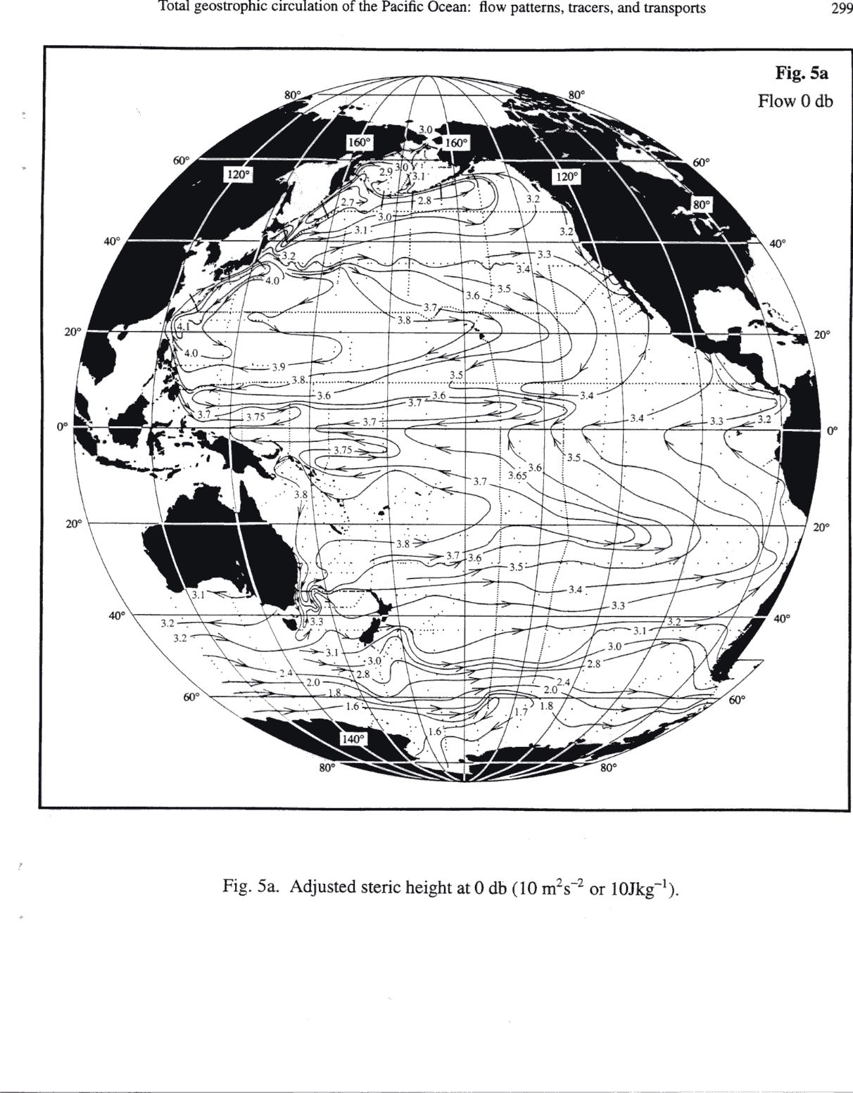
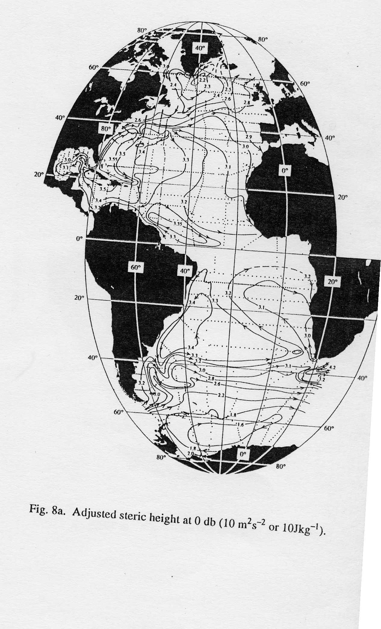
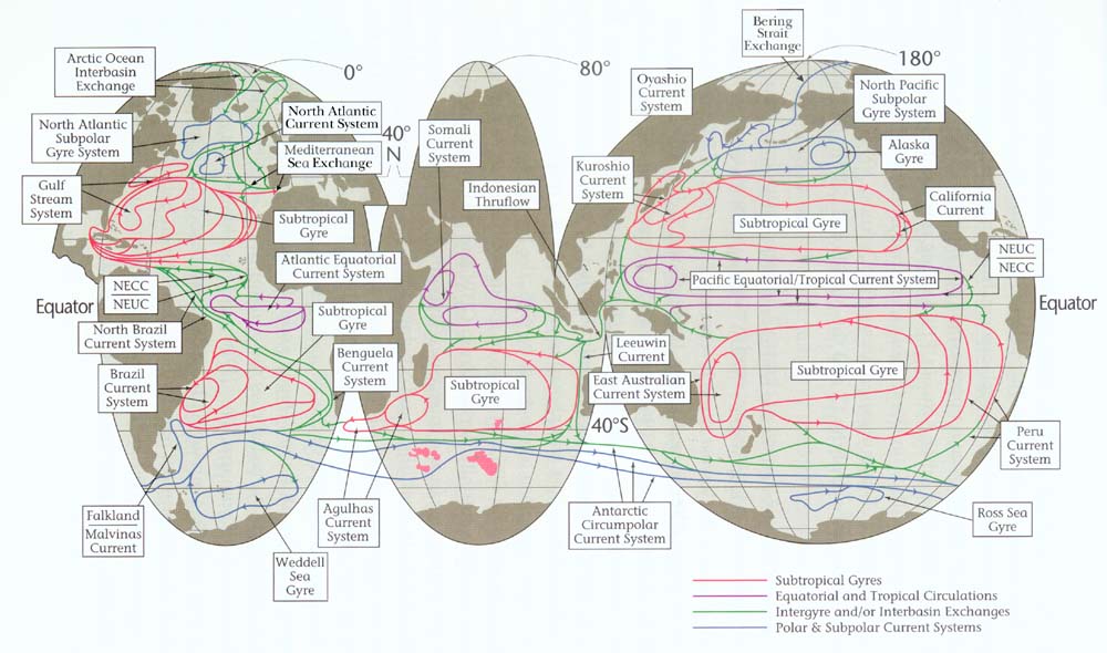
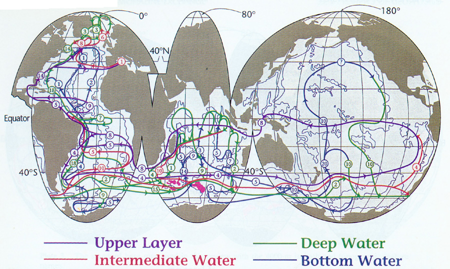
Surface current maps from Reid (1994, 1998), Tomczak and Godfrey text, or Pickard and Emery text show the large-scale geostrophic flow.
Major similarities between the various ocean basins. Note asymmetry of the gyres: strong western boundary currents and weaker flow in the interior; weak and shallow eastern boundary currents.
Subtropical gyres in every ocean basin (high pressure in the middle so flow is clockwise in the northern hemisphere and counterclockwise in the southern hemisphere)
Subpolar gyres in the two northern hemisphere basins and in the Weddell and Ross Seas (low pressure in the middle)
The geostrophic flow in these gyres consists of narrow, swift western boundary currents and gentler flow in the ocean interior away from the western boundary. The western boundary currents and the ACC extend to the ocean bottom. The wind-driven gyre flow in the interior away from the western boundaries extends to about 2000 m depth.
The gyres have eastern boundary currents that apparently extend to no more than about 500 m depth.
There is also an intense wind-driven circulation towards the east around Antarctica, called the Antarctic Circumpolar Current (ACC). It extends to the ocean bottom. It consists of a series of fronts, described in the later lecture on the Southern Ocean.
There are major east-west currents at the equator, which reverse direction every few hundred meters from the top of the ocean to the bottom. (See later lecture on equatorial currents for much better description of these reversing jets, whose vertical scale changes with depth.)
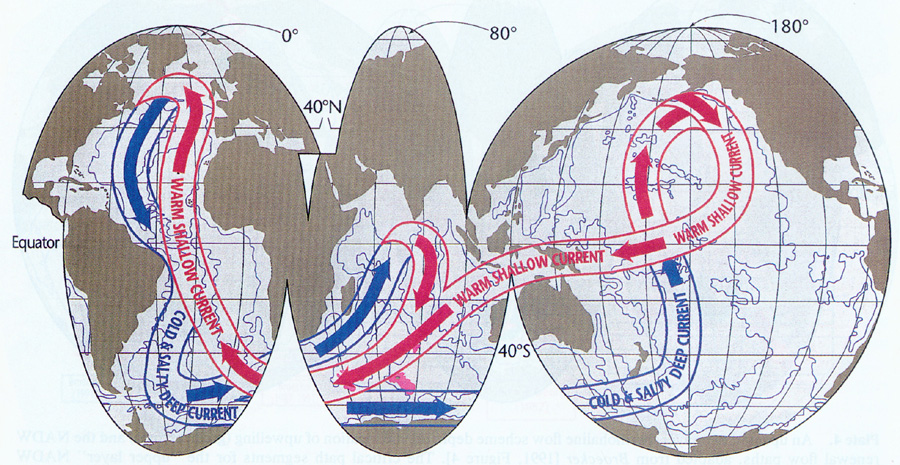
Thermohaline circulation - brief description: Heating/cooling and to a lesser extent evaporation/precipitation drive global and basin-scale circulations characterized by overturn (sinking of dense water and upwelling). The current driven by this are slower than the wind-driven currents in most places. It is useful to think of this circulation as being imposed separately from the wind-driven circulation, although there are likely some nonlinear interactions. Deep western boundary currents and slow interior deep flow are thermohaline.
For a more complete and general description of how the wind drives the general circulation, see:
2.1. Ekman velocity and transport. The wind acts directly and frictionally, through vertical eddy viscosity, on the top 50 to 100 meters of the ocean, in the "Ekman layer". In the northern hemisphere, the frictional surface flow is at an angle to the right of the wind (45 degrees if viscosity is uniform with depth). This frictional surface flow then acts frictionally on the water slightly beneath it, which then is slightly more to the right, etc etc downward with the tips of the vectors tracing a spiral. The frictionally-forced flows become weaker and weaker with depth (exponentially weaker), and die out around 50 to 100 meters down. This spiral is called the "Ekman spiral". The exact details (angle of each successive layer as we move downward through the spiral) of how it spirals depend on the strength and vertical distribution of the vertical eddy viscosity.
If the "transports" are all added up, that is, integrate the velocity over depth at each location, from the bottom to the top of the Ekman layer, the total "Ekman transport" is exactly at right angles to the wind - to the right in the northern hemisphere and left in the southern hemisphere. This direction of the "Ekman transport" is independent of the exact details of the spiral, hence exact details of the vertical eddy viscosity.
The Ekman transport components in the x and y directions (east and
north) are proportional to the wind stress tauy and
taux, in the y and x
directions:
(UEk,VEk) =
(1/rho*f)*(tauy, - taux).
The units are: m2/sec, since this is actually just a velocity
integrated in the vertical direction, and not over an area.
Total Ekman transport across, for instance, a vertical section or line
or curve across the ocean, or around a box, would then be integrated
along the horizontal curve, yielding a complete transport in
m3/sec.
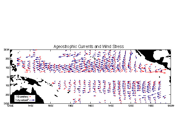
This Ekman effect has been demonstrated by Ralph and Niiler (1999) using surface drifter data from the the Pacific (drogues at 15 m).
Westerlies and trades (see example or Hellerman and Rosenstein [1983] figures in lecture handout or other wind products)
2.2 Sverdrup balance The Ekman layer transports drive circulation in the ocean interior through the Sverdrup transport mechanism. The Ekman layer is the thin frictional layer at the top of the ocean, driven directly by the wind. The whole interior ocean is treated as inviscid, that is without friction. (See study questions for why you can do this.)
Since the wind varies, for instance with latitude (westerlies and trades), the Ekman transport at right angles to the wind also varies. This means there are convergences and divergences in the (horizontal) Ekman transport. Where there is convergence, there must be vertical velocity downward, escaping from the Ekman layer. Where there is divergence, there must be vertical velocity upward, feeding the Ekman transport. We think of these downward and upward velocities as "squashing" or "stretching" the water column beneath the Ekman layer (i.e. most of the ocean depth).
What is the effect of stretching or squashing? The ocean is a rotating fluid (rotating because of the earth). Therefore it has lots of angular momentum. Stretching and squashing act on the angular momentum, like a spinning skater pulling in or spreading out her arms, and hence spinning faster or more slowly. (conservation of angular momentum, involving the rotation rate and the moment of inertia, which has to do with how tall/thin or short/fat the spinning body is).
The only important component of the angular momentum (vorticity) of the ocean water columns is the local vertical component. This is because the water layers involved in the general circulation are very thin and vertically stratified compared with their horizontal extent, so that the horizontal velocities (parallel to surface of earth) are much stronger than the vertical velocities (order cm/sec versus 10^-4^ cm/sec). The angular momentum (vorticity) has two separate and important components - one is due to local "vorticity" in the flow itself (strong eddying) and the other is due to just the rotation of the earth, which gives everything on the earth angular momentum. Thsee two pieces are called the relative vorticity and the planetary vorticity.
In the general circulation, relative vorticity is not important over most of the ocean, with the only notable exceptions being in the very strong western boundary currents and in the east-west equatorial currents. The planetary vorticity (local vertical component) is largest and positive (in the sense of the right-hand rule) at the north pole. It is largest and negative at the south pole. It is zero on the equator. Therefore the important component of the angular momentum increases northward, from large/negative at the south pole through 0 at the equator to large/positive at the north pole.
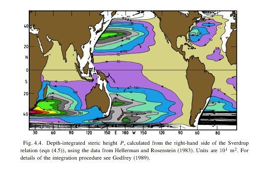
When the frictional Ekman layer exports water downward (very small downward vertical velocity), at the top of the ocean, it squashes the water columns, which must then spin more slowly. This can be accomplished by either spinning more slowly in the location of the water column ("inducing negative relative vorticity"), or moving to another latitude where the local rotation rate (parallel to the local vertical) is slower - this would be equatorward. If on the other hand there is Ekman divergence, then the water columns are "stretched", and the column must spin faster, either in place or by moving to higher latitude. Since the general circulation is very large scale and not filled with ever-increasing vortices, the response is to move in latitude rather than to spin up locally. This response to Ekman pumping or suction is called the "Sverdrup flow". and the flow associated with the response is called "Sverdrup transport". Sverdrup transport is equatorward in subtropical regions of Ekman pumping and poleward in subpolar regions of Ekman suction.
Figure showing Svedrup transport, from Tomczak and Godfrey text
While the direction of Sverdrup flow (equatorward or poleward) is dictated by the Ekman pumping, the flow itself is geostrophic. That is, an equatorward flow means that the sea surface is high in the west and low in the east and vice versa. This is am important point - the force balance is still between pressure gradient force and Coriolis force. The Ekman pumping is a very small and the changes induced in the angular momentum (vorticity) are very weak. These set up the pressure gradient that drives the geostrophic flow. Thus the small terms in the momentum equation, that we neglect in geostrophic balance, are important when thinking about the very slow evolution of the flow or just how the forcing by the Ekman pumping (hence frictional stress of the wind on the sea surface) are communicated to the ocean.
2.3 Western boundary currents. The net Sverdrup transport added up across the ocean (along a parallel of latitude) must be returned in a narrow flow somewhere. The transport of this narrow flow is the same and in the opposite direction to the transport across the whole ocean width; therefore the velocities are much larger than in the ocean interior.
The return flow must ALWAYS be on the western side, regardless of northern or southern hemisphere. Why? Consider the subtropical gyres, where Sverdrup transport is equatorward. The wind through friction is putting "negative" vorticity into the subtropical ocean, through downward Ekman pumping that send the water columns towards lower rotation, e.g. towards the equator. For a steady state, which the general circulation is, this vorticity must be removed somewhere. It is removed through friction in a narrow boundary current. Why "narrow"? Because friction acts best on high gradients of velocity, which you would get in a narrow flow, and because the return flow has to be narrow enough to escape forcing by the Ekman pumping. A frictional boundary current has zero velocity along the boundary, and strong velocity offshore. If the boundary current for the northern hemisphere subtropical gyre is on the west, then the relative vorticity of the boundary current is positive (paddlewheel sense). Thus the frictional boundary current puts positive vorticity into the ocean, which balances the negative vorticity put in by the Ekman pumping. This exact argument works for the low pressure regions as well (subpolar gyre, with northward Sverdrup transport and southward western boundary current). It also works in the southern hemisphere.
The resulting strong, narrow western boundary currents returning all of the interior transport back to the latitude where it started. The Gulf Stream, Kuroshio, Oyashio, Labrador Current, etc etc, presented at the beginning of this lecture, are examples of such wind-driven circulation western boundary currents. Because of various other factors, including just inertia, the western boundary currents are generally stronger than is required to simply return the interior flow. This results in an overshoot of the western boundary current at the latitude where it should end if it were very frictional. Thus the Kuroshio and Gulf Stream, for instance, separate and flow far out to sea before finally dying out.
This topic will be treated in full in the lectures of October 29-November 5. The gross aspects of the salinity and temperature distributions, and the driving force for the slow overturning circulation, are due to surface heating/cooling and surface evaporation/precipitation/ continental runoff. Maps of heat flux and evaporation - precipitation are presented. Components of the heat flux are described (incoming shortwave solar radiation, outgoing longwave radiation, latent heat loss due to evaporation, sensible heat change due to conduction between air and water). Input of fresh water takes place through precipitation and runoff from land. I don't have a net buoyancy flux map for the lecture notes.
Thermohaline forcing takes several forms.
(1) cooling/evaporation
in a region (cooling is often due to
large evaporation), which creates dense water at the sea
surface which then overturns in convective cells. These
cells are very narrow (order 1 km), and are referred to sometimes
as "chimneys", or a whole patch of convective cells might
be referred to as a chimney. Flow in the convective cells
is "ageostrophic" - that is, not geostrophic, since vertical
velocities and vertical length scales are of the same order
as in the horizontal.
(2) Brine rejection resulting
from sea ice formation. This releases salt into the water
column, which increases its density and can create overturn.
(3) Any downward flow due to increase of density must
be compensated somewhere by upwelling and inflow into the
overturning regions. The upwelling must be accompanied
by vertical mixing as the water parcels migrate upward.
This upwelling is an essential part of the thermohaline
circulation and is what forces most of the flow which we
call "thermohaline".
(4) Salt and temperature do not actually mix at exactly the
same rates, especially at the molecular scale - temperature mixes
much faster. This phenomenon is referred to as double diffusion.
This difference in mixing rates can create layering
or overturn - in the ocean, on vertical scales of several to 10's
of meters. This is a form of thermohaline forcing.
3.1.Buoyancy forcing.
Annual mean net evaporation minus precipitation (cm/yr)
NCEP map of annual mean evaporation minus precipitation (cm/yr).
Indirect #1. Use estimates of the heat flux at the sea surface
from the atmosphere to the ocean. These fluxes are calculated as a sum
of the incoming solar radiation (based on earth orbit and cloudiness),
loss of heat due to evaporation since evaporation takes work and hence
removes energy from the ocean ("latent heat flux"), exchange of heat due
to temperature difference between air and water right at the air-sea
interface ("sensible heat flux"), and loss of heat due to back radiation
from the ocean to the atmosphere (similar to black body radiation).
Using the net air-sea flux in Watts/(meter^2) over an area, calculate
the net heat exchange in Watts by summing the flux over the area.
Then the net heat transport by the ocean across the closed box
surrounding that area is equal to the net heat exchange out of the
surface of the box. (Assuming that geothermal flux from the ocean
bottom is negligible, which it is.)
Common method for doing this: integrate air-sea heat flux across
latitude bands to get the net ocean heat transport across those
latitudes.
Indirect #2. Use calculations of the net heat exchange between
space and the very top of the atmosphere, and direct estimates of net
heat transport across latitude bands in the atmosphere (based on
atmosphere winds and temperatures). Subtract atmosphere's heat transport
from the net earth-space estimate to get the ocean heat transport
across the latitude (all the way around the earth - not possible to
separate oceans).
3.3. Thermohaline circulation.
The factors that affect buoyancy (density) at the sea surface (and to a much
lesser extent the direct factors in the ocean interior such as geothermal
heating) drive a circulation, called the thermohaline circulation. Our simple
picture of this is that there are quite isolated sources of deeper waters -
that is, that convection due to loss of buoyancy (gain of density) at the sea
surface, are very localized. Examples are small regions in the Greenland
Sea, Mediterranean Sea, Labrador Sea, Weddell Sea, Japan Sea, etc. and
areas of dense shelf water formation due to sea ice formation. These
newly-formed deeper waters sink and fill the oceans at depth. The result
must be upwelling of these waters. We are still working as a community on
exactly where the upwelling occurs. We assume it is very widespread,
although there may be some local areas of more intense upwelling such as the
equator. With widespread upwelling, the deep water columns are stretched.
The deep water then responds in a fashion much like the Sverdrup response to
Ekman pumping - the water columns "stretch" and must therefore move poleward.
The net result is that the deep circulation should be more or less cyclonic
(counterclockwise northern hemisphere, clockwise southern hemisphere, with
low pressure in the center).
On a more global scale, there is a net transport of upper layer water into the isolated
water mass formation sites and net transport of lower layer water away from
the isolated sites. This is accomplished through a combination of the gentle
deep gyres of the previous paragraphs, and western boundary currents that
complete the mass balance.
The overall thermohaline circulation is about 1/10 the magnitude of the
wind-driven circulation. That is, the net transports associated with it are
on the order of 10-20 Sverdrups. However, the THC extends to the ocean
bottom, whereas the wind-driven circulation by and large does not (except in
the strong western boundary currents and Antarctic Circumpolar Current, where
it does go to the bottom). Therefore almost all of the interior ocean
circulation seen below about 2000 m is due to thermohaline forcing.
Annual mean net heat flux (W/m2)
ECMWF map of surface heat flux (W/m2)
(positive means heat into ocean)
from Bernard Barnier, using
the European Center for Medium Range Weather
Forecasting analyses for the years 1986-1988 to compute surface fluxes.
Fields were made available by
Barnier for this map which reproduces a similar map in
the following reference:
Barnier, B., L. Siefridt and P. Marchesiello, 1994. Thermal
forcing for a global ocean circulation model using a three-
year climatology of ECMWF analyses. J. Marine Systems, 6,
363-380.
Annual mean E-P
in cm/year constructed
from climatology data in DaSilva's online
Atlas of Surface Marine Data, from:
DaSilva, A. M., C. C. Young and S. Levitus, 1994. Atlas of surface
marine data 1994.
3.2. Heat transport estimates.
Heat transport was defined above in section 1.3. We calculate it for the
ocean in three ways.
Typically we calculate the transports across a given latitude for each
ocean - it is easiest to understand the following calculations if you
think about them this way first. Of course the direct and indirect #1
estimates described below can also be done for any closed box (surface
area) of the ocean.
Direct.Calculate the integral given in section 1.3 for a vertical
section (or closed box surrounded by vertical planes)
using measurements of temperature (and salinity in
order to calculate density, specific heat and potential temperature)
and estimate of velocity, usually based on geostrophy and assumptions
about the unknown reference velocities. The quantity is only useful
if mass is balanced across the vertical section, which must therefore be
a closed box. The "box" can be closed by being a section which goes
from one coast to another (so could be a straight line across an ocean),
or it could be a closed box within the ocean. (Why is heat transport
only useful if mass is balanced?). In practice this can only be done
well where geostrophic velocities are well constrained.